Visualize Your Data
To understand our data, we will look for correlations between features and the label. This can be important when choosing a model. E.g., if features and a label are linearly correlated, a linear model like Linear Regression can do well; if the relationship is very non-linear, more complex models such as Decision Trees can be better. We can use Databrick’s built in visualization to view each of our predictors in relation to the label column as a scatter plot to see the correlation between the predictors and the label.
Exploratory Data Analysis (EDA) is an approach/philosophy for data analysis that employs a variety of techniques (mostly graphical) to
- maximize insight into a data set;
- uncover underlying structure;
- extract important variables;
- detect outliers and anomalies;
- test underlying assumptions;
- develop parsimonious models; and
- determine optimal factor settings.

Temperature VS Power
%sql

select AT as Temperature, PE as Power from PowerPlant


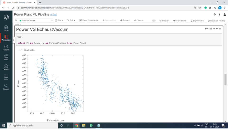
Power VS Exhaust Vaccum
%sql

select PE as Power, V as ExhaustVaccum from PowerPlant


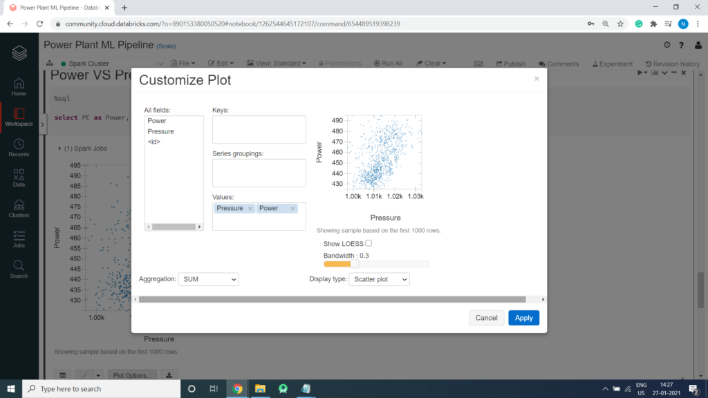
Power VS Pressure
%sql

select PE as Power, AP as Pressure from PowerPlant

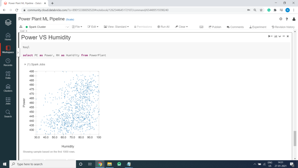
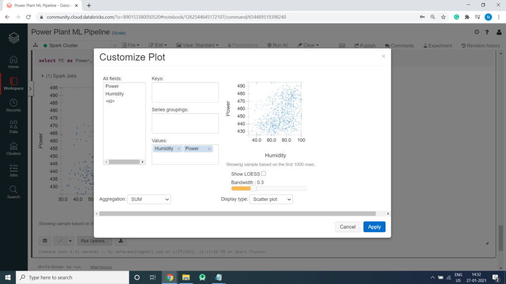
Power VS Humidity
%sql

select PE as Power, RH as Humidity from PowerPlant
Split the Data
It is common practice when building machine learning models to split the source data, using some of it to train the model and reserving some to test the trained model. In this project, you will use 70% of the data for training, and reserve 30% for testing.
%scala

val splits = csv.randomSplit(Array(0.7, 0.3))
val train = splits(0)
val test = splits(1)
val train_rows = train.count()
val test_rows = test.count()
println("Training Rows: " + train_rows + " Testing Rows: " + test_rows)
Prepare the Training Data
To train the Regression model, you need a training data set that includes a vector of numeric features, and a label column. In this project, you will use the VectorAssembler class to transform the feature columns into a vector, and then rename the PE column to the label.
VectorAssembler()
VectorAssembler(): is a transformer that combines a given list of columns into a single vector column. It is useful for combining raw features and features generated by different feature transformers into a single feature vector, in order to train ML models like logistic regression and decision trees.
VectorAssembler accepts the following input column types: all numeric types, boolean type, and vector type.
In each row, the values of the input columns will be concatenated into a vector in the specified order.
%scala

import org.apache.spark.ml.feature.VectorAssembler

val assembler = new VectorAssembler().setInputCols(Array("AT", "V", "AP", "RH")).setOutputCol("features")

val training = assembler.transform(train).select($"features", $"PE".alias("label"))

training.show(false)

Output:

+--------------------------+------+
|features                  |label |
+--------------------------+------+
|[1.81,39.42,1026.92,76.97]|490.55|
|[2.34,39.42,1028.47,69.68]|490.34|
|[2.64,39.64,1011.02,85.24]|481.29|
|[2.71,39.42,1026.66,81.11]|489.3 |
|[3.0,39.64,1011.0,80.14]  |485.2 |
|[3.21,38.44,1016.9,86.34] |491.35|
|[3.21,38.44,1017.11,84.86]|492.93|
|[3.26,41.31,996.32,100.0] |489.38|
|[3.38,41.31,998.79,97.76] |489.11|
|[3.51,35.47,1017.53,86.56]|489.07|
|[3.6,35.19,1018.73,99.1]  |488.98|
|[3.68,39.64,1011.31,84.05]|490.02|
|[3.73,39.42,1024.4,82.42] |488.58|
|[3.91,35.47,1016.92,86.03]|488.67|
|[3.92,41.31,999.22,95.26] |487.35|
|[3.94,39.9,1008.06,97.49] |488.81|
|[3.95,35.47,1017.36,84.88]|488.64|
|[3.95,38.44,1016.75,79.65]|492.46|
|[3.98,35.47,1017.22,86.53]|489.64|
|[3.99,39.64,1011.53,83.58]|492.06|
+--------------------------+------+
only showing top 20 rows
Train a Regression Model
Next, you need to train a Regression model using the training data. To do this, create an instance of the Linear Regression algorithm you want to use and use its fit method to train a model based on the training DataFrame. In this project, you will use a Logistic Regression Classifier algorithm – though you can use the same technique for any of the regression algorithms supported in the spark.ml API
%scala

import org.apache.spark.ml.regression.LinearRegression

val lr = new LinearRegression().setLabelCol("label").setFeaturesCol("features").setMaxIter(10).setRegParam(0.3)
val model = lr.fit(training)
println("Model Trained!")
Prepare the Testing Data
Now that you have a trained model, you can test it using the testing data you reserved previously. First, you need to prepare the testing data in the same way as you did the training data by transforming the feature columns into a vector. This time you’ll rename the PE column to trueLabel.
%scala

val testing = assembler.transform(test).select($"features", $"PE".alias("trueLabel"))
testing.show(false)

Output:

+--------------------------+---------+
|features                  |trueLabel|
+--------------------------+---------+
|[2.58,39.42,1028.68,69.03]|488.69   |
|[2.8,39.64,1011.01,82.96] |482.66   |
|[3.2,41.31,997.67,98.84]  |489.86   |
|[3.31,39.42,1024.05,84.31]|487.19   |
|[3.38,39.64,1011.0,81.22] |488.92   |
|[3.4,39.64,1011.1,83.43]  |459.86   |
|[3.63,38.44,1016.16,87.38]|487.87   |
|[3.69,38.44,1016.74,82.87]|490.78   |
|[3.74,35.19,1018.58,98.84]|490.5    |
|[3.82,35.47,1016.62,84.34]|489.04   |
|[3.85,35.47,1016.78,85.31]|489.78   |
|[3.96,35.47,1016.79,83.81]|489.68   |
|[4.04,35.47,1017.51,87.35]|486.86   |
|[4.08,35.19,1018.87,97.07]|489.44   |
|[4.15,39.9,1008.84,96.68] |491.22   |
|[4.16,35.47,1017.72,88.49]|486.7    |
|[4.24,39.9,1009.28,96.74] |491.25   |
|[4.27,39.64,1010.99,84.85]|487.19   |
|[4.32,35.47,1017.8,88.51] |488.03   |
|[4.69,39.42,1024.58,79.35]|486.34   |
+--------------------------+---------+
only showing top 20 rows
Test the Model
Now you’re ready to use the transform method of the model to generate some predictions. You can use this approach to predict the PE; but in this case, you are using the test data which includes a known true label value, so you can compare the PE
%scala

val prediction = model.transform(testing)
val predicted = prediction.select("features", "prediction", "trueLabel")
predicted.show()

Output:

+--------------------+------------------+---------+
|            features|        prediction|trueLabel|
+--------------------+------------------+---------+
|[2.58,39.42,1028....|  491.859574767746|   488.69|
|[2.8,39.64,1011.0...| 487.7161757678857|   482.66|
|[3.2,41.31,997.67...| 483.0465542807676|   489.86|
|[3.31,39.42,1024....|488.08275616778946|   487.19|
|[3.38,39.64,1011....| 486.8822847729832|   488.92|
|[3.4,39.64,1011.1...| 486.5745301394958|   459.86|
|[3.63,38.44,1016....|  486.540697435181|   487.87|
|[3.69,38.44,1016....|487.06975735358276|   490.78|
|[3.74,35.19,1018....|486.07023009996726|    490.5|
|[3.82,35.47,1016....|  487.484601260791|   489.04|
|[3.85,35.47,1016....| 487.3234200396172|   489.78|
|[3.96,35.47,1016....|487.31591675628243|   489.68|
|[4.04,35.47,1017....| 486.7959634355635|   486.86|
|[4.08,35.19,1018....|485.70898895188856|   489.44|
|[4.15,39.9,1008.8...| 483.2009943494979|   491.22|
|[4.16,35.47,1017....|486.45476108622137|    486.7|
|[4.24,39.9,1009.2...| 483.0769908980244|   491.25|
|[4.27,39.64,1010....|484.79897907459224|   487.19|
|[4.32,35.47,1017....| 486.1697967448147|   488.03|
|[4.69,39.42,1024....| 486.2629590924871|   486.34|
+--------------------+------------------+---------+
only showing top 20 rows
Examine the Predicted and Actual Values
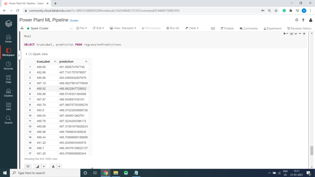
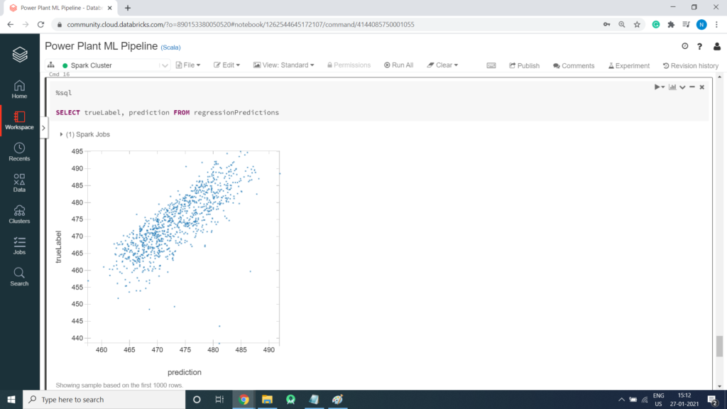
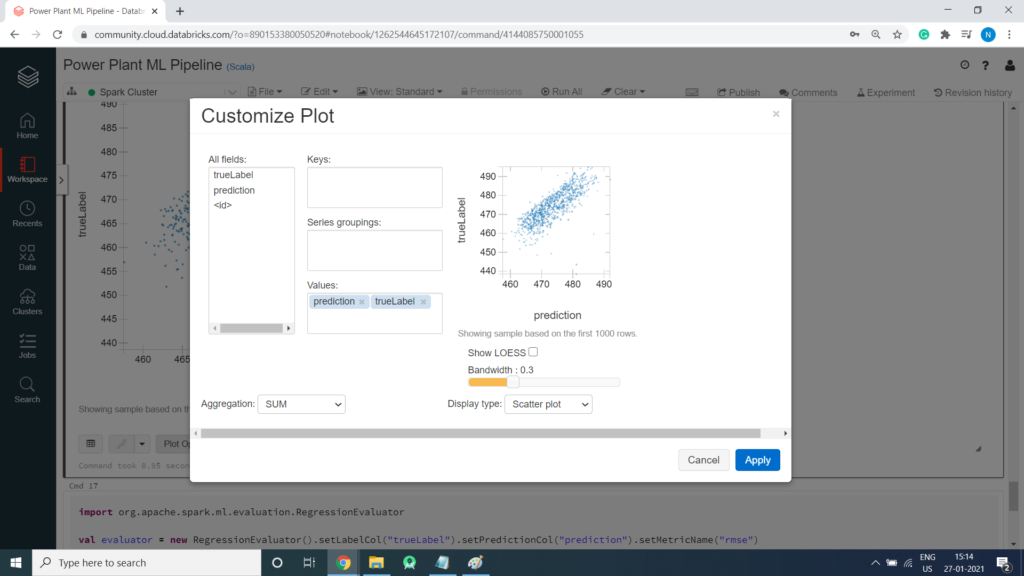
You can plot the predicted values against the actual values to see how accurately the model has predicted. In a perfect model, the resulting scatter plot should form a perfect diagonal line with each predicted value being identical to the actual value – in practice, some variance is to be expected. Run the cells below to create a temporary table from the predicted DataFrame and then retrieve the predicted and actual label values using SQL. You can then display the results as a scatter plot, specifying – as the function to show the unaggregated values.
%scala

predicted.createOrReplaceTempView("regressionPredictions")
%sql SELECT trueLabel, prediction FROM regressionPredictions
Scatter Plot creation
Retrieve the Root Mean Square Error (RMSE)
There are a number of metrics used to measure the variance between predicted and actual values. Of these, the root mean square error (RMSE) is a commonly used value that is measured in the same units as the predicted and actual values – so in this case, the RMSE indicates the average number of minutes between predicted and actual PE values. You can use the RegressionEvaluator class to retrieve the RMSE.
import org.apache.spark.ml.evaluation.RegressionEvaluator

val evaluator = new RegressionEvaluator().setLabelCol("trueLabel").setPredictionCol("prediction").setMetricName("rmse")
val rmse = evaluator.evaluate(prediction)
println("Root Mean Square Error (RMSE): " + (rmse))

Output:

Root Mean Square Error (RMSE): 4.636465739523349
import org.apache.spark.ml.evaluation.RegressionEvaluator
evaluator: org.apache.spark.ml.evaluation.RegressionEvaluator = RegressionEvaluator: uid=regEval_5e0c8129af2e, metricName=rmse, throughOrigin=false
rmse: Double = 4.636465739523349