
Customer segmentation is the practice of dividing a company’s customers into groups that reflect similarities among customers in each group. The goal of segmenting customers is to decide how to relate to customers in each segment in order to maximize the value of each customer to the business.
Problem Statement or Business Problem
In this project, we will perform one of the most essential applications of machine learning – Customer Segmentation. We will implement customer segmentation in Apache Spark and Scala, whenever you need to find your best customer.
Customer Segmentation is one of the most important applications of unsupervised learning. In this machine learning project, we will make use of K-means clustering which is the essential algorithm for clustering unlabeled datasets.
Attribute Information or Dataset Details:
- CustomerID
- Gender
- Age
- Annual Income (k$)
- Spending Score (1-100)
Technology Used
- Apache Spark
- Spark SQL
- Apache Spark MLLib
- Scala
- DataFrame-based API
- Apache Zeppelin Notebook
Introduction
Welcome to this project on Customer Segmentation using Apache Spark Machine Learning using Apache Zeppelin platform which allows you to execute your spark code in Apache Zeppelin notebook.
In this project, we explore Apache Spark and Machine Learning on Apache Zeppelin.
I am a firm believer that the best way to learn is by doing. That’s why I haven’t included any purely theoretical lectures in this tutorial: you will learn everything on the way and be able to put it into practice straight away. Seeing the way each feature works will help you learn Apache Spark machine learning thoroughly by heart.
We’re going to look at how to set up Apache Spark on Apache Zeppelin and get started with that. And we’ll look at how we can then use Apache Spark and process that data using a Machine Learning model, and generate some sort of output in the form of a prediction. That’s pretty much what we’re going to learn about the predictive model.
In this project, we will be creating Customer Segmentation using Mall data. We will make use of K-means clustering which is the essential algorithm for clustering unlabeled datasets.
We will learn:
- Preparing the Data for Processing.
- Basics flow of data in Apache Spark, loading data, and working with data, this course shows you how Apache Spark is perfect for a Machine Learning job.
- Learn the basics of Apache Zeppelin
- Define the Machine Learning Pipeline
- Train a Machine Learning Model
- Testing a Machine Learning Model
- Evaluating a Machine Learning Model (i.e. Examine the Predicted and Actual Values)
- The goal is to provide you with practical tools that will be beneficial for you in the future. While doing that, you’ll develop a model with a real use opportunity.
I am really excited you are here, I hope you are going to follow all the way to the end of the Project. It is fairly straight forward fairly easy to follow through the article we will show you step by step each line of code & we will explain what it does and why we are doing it.
Apache Zeppelin with Apache Spark Installation on Ubuntu
Download Data
Click Here
Load Data in Dataframe
We are loading CSV (.csv) file into Apache Spark Dataframe
%spark

// File location and type
val file_location = "/home/bigdata/files/Mall_Customers.csv"
val file_type = "csv"

// CSV options
val infer_schema = "true"
val first_row_is_header = "true"
val delimiter = ","

// The applied options are for CSV files. For other file types, these will be ignored.
val mallDataDF = spark.read.format(file_type)
  .option("inferSchema", infer_schema)
  .option("header", first_row_is_header)
  .option("sep", delimiter)
  .load(file_location)

mallDataDF.show()

Output:

+----------+------+---+------------------+----------------------+
|CustomerID|Gender|Age|Annual Income (k$)|Spending Score (1-100)|
+----------+------+---+------------------+----------------------+
|         1|  Male| 19|                15|                    39|
|         2|  Male| 21|                15|                    81|
|         3|Female| 20|                16|                     6|
|         4|Female| 23|                16|                    77|
|         5|Female| 31|                17|                    40|
|         6|Female| 22|                17|                    76|
|         7|Female| 35|                18|                     6|
|         8|Female| 23|                18|                    94|
|         9|  Male| 64|                19|                     3|
|        10|Female| 30|                19|                    72|
|        11|  Male| 67|                19|                    14|
|        12|Female| 35|                19|                    99|
|        13|Female| 58|                20|                    15|
|        14|Female| 24|                20|                    77|
|        15|  Male| 37|                20|                    13|
|        16|  Male| 22|                20|                    79|
|        17|Female| 35|                21|                    35|
|        18|  Male| 20|                21|                    66|
|        19|  Male| 52|                23|                    29|
|        20|Female| 35|                23|                    98|
+----------+------+---+------------------+----------------------+
only showing top 20 rows
Get Statistics of Data
%spark


mallDataDF.describe().show()

Output:

+-------+------------------+------+-----------------+------------------+----------------------+
|summary|        CustomerID|Gender|              Age|Annual Income (k$)|Spending Score (1-100)|
+-------+------------------+------+-----------------+------------------+----------------------+
|  count|               200|   200|              200|               200|                   200|
|   mean|             100.5|  null|            38.85|             60.56|                  50.2|
| stddev|57.879184513951124|  null|13.96900733155888| 26.26472116527124|    25.823521668370173|
|    min|                 1|Female|               18|                15|                     1|
|    max|               200|  Male|               70|               137|                    99|
+-------+------------------+------+-----------------+------------------+----------------------+
Printing Schema of Dataframe
%spark


mallDataDF.printSchema()

Output:

root
 |-- CustomerID: integer (nullable = true)
 |-- Gender: string (nullable = true)
 |-- Age: integer (nullable = true)
 |-- Annual Income (k$): integer (nullable = true)
 |-- Spending Score (1-100): integer (nullable = true)
Create Temporary View so we can perform Spark SQL on Data
%spark

mallDataDF.createOrReplaceTempView("MallData");
Exploratory Data Analysis or EDA
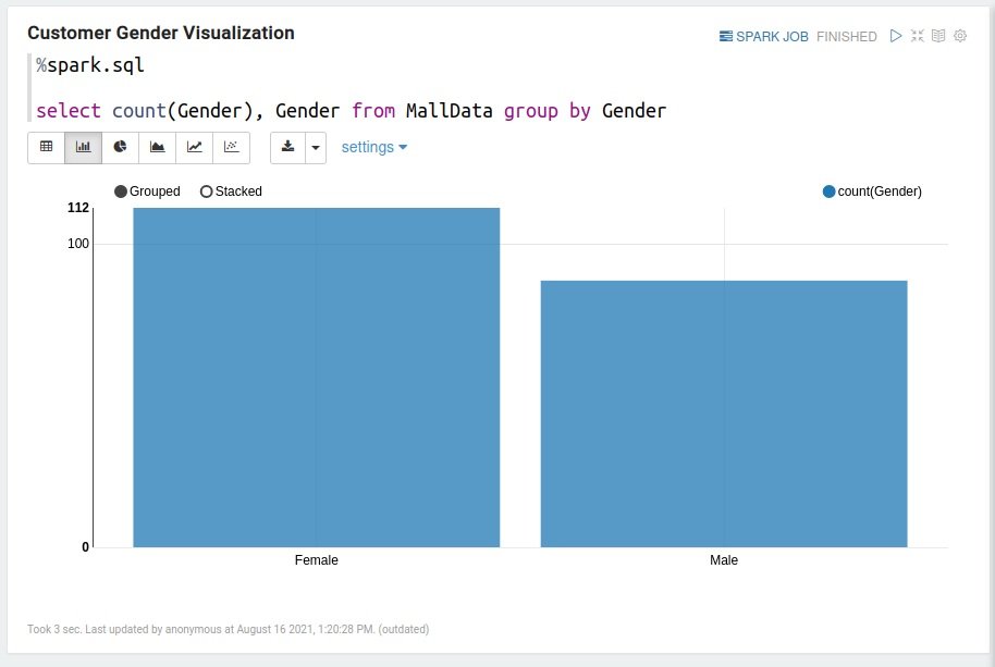
Customer Gender Visualization
%spark.sql

select count(Gender), Gender from MallData group by Gender
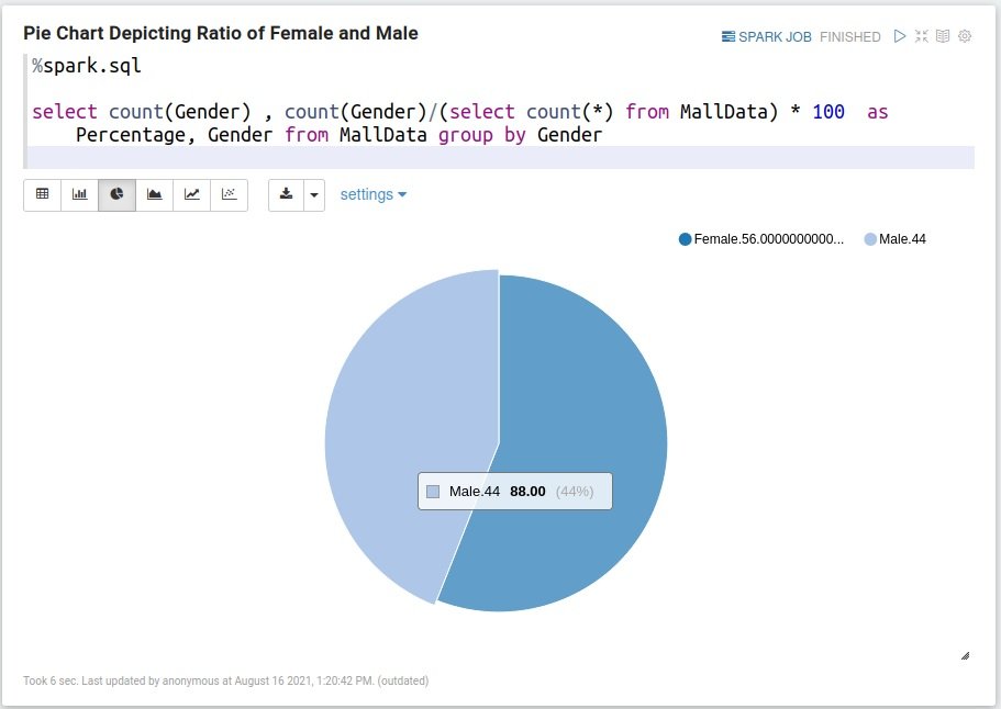
Pie Chart Depicting Ratio of Female and Male
%spark.sql

select count(Gender) , count(Gender)/(select count(*) from MallData) * 100  as Percentage, Gender from MallData group by Gender
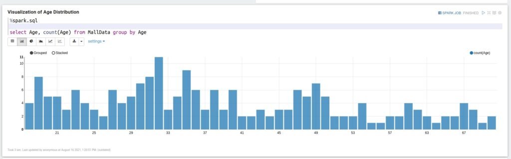
Visualization of Age Distribution
%spark.sql

select Age, count(Age) from MallData group by Age
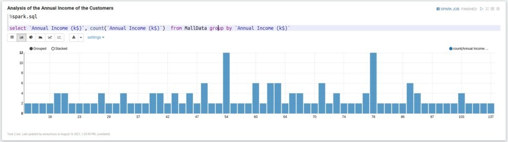
Analysis of the Annual Income of the Customers
%spark.sql

select `Annual Income (k$)`, count(`Annual Income (k$)`)  from MallData group by `Annual Income (k$)`
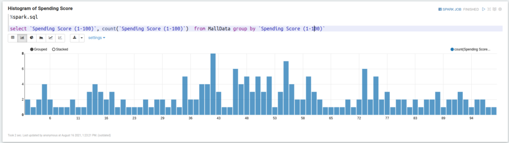
Histogram of Spending Score
%spark.sql

select `Spending Score (1-100)`, count(`Spending Score (1-100)`)  from MallData group by `Spending Score (1-100)`
Define the Pipeline
A predictive model often requires multiple stages of feature preparation.
A pipeline consists of a series of transformer and estimator stages that typically prepare a DataFrame for modeling and then train a predictive model.
In this case, you will create a pipeline with stages:
- A StringIndexer estimator that converts string values to indexes for categorical features
- A VectorAssembler that combines categorical features into a single vector
Split the Data
It is common practice when building machine learning models to split the source data, using some of it to train the model and reserving some to test the trained model. In this project, you will use 70% of the data for training, and reserve 30% for testing.
%spark

val splits = mallDataDF.randomSplit(Array(0.7, 0.3))
val train = splits(0)
val test = splits(1)
val train_rows = train.count()
val test_rows = test.count()
println("Training Rows: " + train_rows + " Testing Rows: " + test_rows)
Prepare the Training Data
To train the K means cluster model, you need a training data set that includes a vector of numeric features, and a label column. In this project, you will use the VectorAssembler class to transform the feature columns into a vector.
%spark

import org.apache.spark.ml.feature.VectorAssembler

val assembler = new VectorAssembler().setInputCols(Array("Annual Income (k$)", "Spending Score (1-100)")).setOutputCol("features")

val training = assembler.transform(train)

training.show()

Output:

+----------+------+---+------------------+----------------------+-----------+
|CustomerID|Gender|Age|Annual Income (k$)|Spending Score (1-100)|   features|
+----------+------+---+------------------+----------------------+-----------+
|         1|  Male| 19|                15|                    39|[15.0,39.0]|
|         3|Female| 20|                16|                     6| [16.0,6.0]|
|         4|Female| 23|                16|                    77|[16.0,77.0]|
|         6|Female| 22|                17|                    76|[17.0,76.0]|
|         7|Female| 35|                18|                     6| [18.0,6.0]|
|         8|Female| 23|                18|                    94|[18.0,94.0]|
|         9|  Male| 64|                19|                     3| [19.0,3.0]|
|        10|Female| 30|                19|                    72|[19.0,72.0]|
|        11|  Male| 67|                19|                    14|[19.0,14.0]|
|        12|Female| 35|                19|                    99|[19.0,99.0]|
|        17|Female| 35|                21|                    35|[21.0,35.0]|
|        19|  Male| 52|                23|                    29|[23.0,29.0]|
|        20|Female| 35|                23|                    98|[23.0,98.0]|
|        22|  Male| 25|                24|                    73|[24.0,73.0]|
|        23|Female| 46|                25|                     5| [25.0,5.0]|
|        25|Female| 54|                28|                    14|[28.0,14.0]|
|        27|Female| 45|                28|                    32|[28.0,32.0]|
|        28|  Male| 35|                28|                    61|[28.0,61.0]|
|        29|Female| 40|                29|                    31|[29.0,31.0]|
|        30|Female| 23|                29|                    87|[29.0,87.0]|
+----------+------+---+------------------+----------------------+-----------+
only showing top 20 rows

import org.apache.spark.ml.feature.VectorAssembler
assembler: org.apache.spark.ml.feature.VectorAssembler = vecAssembler_7cedfd618a51
training: org.apache.spark.sql.DataFrame = [CustomerID: int, Gender: string ... 4 more fields]
Train a K-Means Cluster Model
Next, you need to train a K Means Cluster model using the training data.
%spark

import org.apache.spark.ml.clustering.KMeans

val kmeans = new KMeans()
  .setK(5)
  .setFeaturesCol("features")
  .setPredictionCol("prediction")

val kmeansModel = kmeans.fit(training)

Output:

import org.apache.spark.ml.clustering.KMeans
kmeans: org.apache.spark.ml.clustering.KMeans = kmeans_9acb8f8d4f3c
kmeansModel: org.apache.spark.ml.clustering.KMeansModel = kmeans_9acb8f8d4f3c
Prepare the Testing Data
Now that you have a trained model, you can test it using the testing data you reserved previously. First, you need to prepare the testing data in the same way as you did the training data by transforming the feature columns into a vector.
%spark

val testing = assembler.transform(test)

testing.show()

Output:

+----------+------+---+------------------+----------------------+-----------+
|CustomerID|Gender|Age|Annual Income (k$)|Spending Score (1-100)|   features|
+----------+------+---+------------------+----------------------+-----------+
|         2|  Male| 21|                15|                    81|[15.0,81.0]|
|         5|Female| 31|                17|                    40|[17.0,40.0]|
|        13|Female| 58|                20|                    15|[20.0,15.0]|
|        14|Female| 24|                20|                    77|[20.0,77.0]|
|        15|  Male| 37|                20|                    13|[20.0,13.0]|
|        16|  Male| 22|                20|                    79|[20.0,79.0]|
|        18|  Male| 20|                21|                    66|[21.0,66.0]|
|        21|  Male| 35|                24|                    35|[24.0,35.0]|
|        24|  Male| 31|                25|                    73|[25.0,73.0]|
|        26|  Male| 29|                28|                    82|[28.0,82.0]|
|        31|  Male| 60|                30|                     4| [30.0,4.0]|
|        40|Female| 20|                37|                    75|[37.0,75.0]|
|        41|Female| 65|                38|                    35|[38.0,35.0]|
|        44|Female| 31|                39|                    61|[39.0,61.0]|
|        46|Female| 24|                39|                    65|[39.0,65.0]|
|        51|Female| 49|                42|                    52|[42.0,52.0]|
|        54|  Male| 59|                43|                    60|[43.0,60.0]|
|        56|  Male| 47|                43|                    41|[43.0,41.0]|
|        58|  Male| 69|                44|                    46|[44.0,46.0]|
|        65|  Male| 63|                48|                    51|[48.0,51.0]|
+----------+------+---+------------------+----------------------+-----------+
only showing top 20 rows

testing: org.apache.spark.sql.DataFrame = [CustomerID: int, Gender: string ... 4 more fields]
Test the Model
Now you’re ready to use the transform method of the model to generate some predictions.
%spark

val prediction = kmeansModel.transform(testing)

prediction.show(100)

Output:

+----------+------+---+------------------+----------------------+------------+----------+
|CustomerID|Gender|Age|Annual Income (k$)|Spending Score (1-100)|    features|prediction|
+----------+------+---+------------------+----------------------+------------+----------+
|         2|  Male| 21|                15|                    81| [15.0,81.0]|         1|
|         5|Female| 31|                17|                    40| [17.0,40.0]|         0|
|        13|Female| 58|                20|                    15| [20.0,15.0]|         0|
|        14|Female| 24|                20|                    77| [20.0,77.0]|         1|
|        15|  Male| 37|                20|                    13| [20.0,13.0]|         0|
|        16|  Male| 22|                20|                    79| [20.0,79.0]|         1|
|        18|  Male| 20|                21|                    66| [21.0,66.0]|         1|
|        21|  Male| 35|                24|                    35| [24.0,35.0]|         0|
|        24|  Male| 31|                25|                    73| [25.0,73.0]|         1|
|        26|  Male| 29|                28|                    82| [28.0,82.0]|         1|
|        31|  Male| 60|                30|                     4|  [30.0,4.0]|         0|
|        40|Female| 20|                37|                    75| [37.0,75.0]|         1|
|        41|Female| 65|                38|                    35| [38.0,35.0]|         0|
|        44|Female| 31|                39|                    61| [39.0,61.0]|         4|
|        46|Female| 24|                39|                    65| [39.0,65.0]|         1|
|        51|Female| 49|                42|                    52| [42.0,52.0]|         4|
|        54|  Male| 59|                43|                    60| [43.0,60.0]|         4|
|        56|  Male| 47|                43|                    41| [43.0,41.0]|         4|
|        58|  Male| 69|                44|                    46| [44.0,46.0]|         4|
|        65|  Male| 63|                48|                    51| [48.0,51.0]|         4|
|        66|  Male| 18|                48|                    59| [48.0,59.0]|         4|
|        69|  Male| 19|                48|                    59| [48.0,59.0]|         4|
|        71|  Male| 70|                49|                    55| [49.0,55.0]|         4|
|        77|Female| 45|                54|                    53| [54.0,53.0]|         4|
|        80|Female| 49|                54|                    42| [54.0,42.0]|         4|
|        81|  Male| 57|                54|                    51| [54.0,51.0]|         4|
|        89|Female| 34|                58|                    60| [58.0,60.0]|         4|
|        90|Female| 50|                58|                    46| [58.0,46.0]|         4|
|        92|  Male| 18|                59|                    41| [59.0,41.0]|         4|
|        93|  Male| 48|                60|                    49| [60.0,49.0]|         4|
|       101|Female| 23|                62|                    41| [62.0,41.0]|         4|
|       102|Female| 49|                62|                    48| [62.0,48.0]|         4|
|       106|Female| 21|                62|                    42| [62.0,42.0]|         4|
|       107|Female| 66|                63|                    50| [63.0,50.0]|         4|
|       108|  Male| 54|                63|                    46| [63.0,46.0]|         4|
|       111|  Male| 65|                63|                    52| [63.0,52.0]|         4|
|       113|Female| 38|                64|                    42| [64.0,42.0]|         4|
|       114|  Male| 19|                64|                    46| [64.0,46.0]|         4|
|       120|Female| 50|                67|                    57| [67.0,57.0]|         4|
|       121|  Male| 27|                67|                    56| [67.0,56.0]|         4|
|       126|Female| 31|                70|                    77| [70.0,77.0]|         3|
|       127|  Male| 43|                71|                    35| [71.0,35.0]|         4|
|       129|  Male| 59|                71|                    11| [71.0,11.0]|         2|
|       130|  Male| 38|                71|                    75| [71.0,75.0]|         3|
|       132|  Male| 39|                71|                    75| [71.0,75.0]|         3|
|       139|  Male| 19|                74|                    10| [74.0,10.0]|         2|
|       140|Female| 35|                74|                    72| [74.0,72.0]|         3|
|       141|Female| 57|                75|                     5|  [75.0,5.0]|         2|
|       142|  Male| 32|                75|                    93| [75.0,93.0]|         3|
|       144|Female| 32|                76|                    87| [76.0,87.0]|         3|
|       151|  Male| 43|                78|                    17| [78.0,17.0]|         2|
|       152|  Male| 39|                78|                    88| [78.0,88.0]|         3|
|       156|Female| 27|                78|                    89| [78.0,89.0]|         3|
|       158|Female| 30|                78|                    78| [78.0,78.0]|         3|
|       173|  Male| 36|                87|                    10| [87.0,10.0]|         2|
|       174|  Male| 36|                87|                    92| [87.0,92.0]|         3|
|       175|Female| 52|                88|                    13| [88.0,13.0]|         2|
|       177|  Male| 58|                88|                    15| [88.0,15.0]|         2|
|       182|Female| 32|                97|                    86| [97.0,86.0]|         3|
|       183|  Male| 46|                98|                    15| [98.0,15.0]|         2|
|       186|  Male| 30|                99|                    97| [99.0,97.0]|         3|
|       190|Female| 36|               103|                    85|[103.0,85.0]|         3|
|       198|  Male| 32|               126|                    74|[126.0,74.0]|         3|
|       199|  Male| 32|               137|                    18|[137.0,18.0]|         2|
+----------+------+---+------------------+----------------------+------------+----------+

prediction: org.apache.spark.sql.DataFrame = [CustomerID: int, Gender: string ... 5 more fields]
%spark

prediction.groupBy("prediction").count().show()

Output:

+----------+-----+
|prediction|count|
+----------+-----+
|         1|    8|
|         3|   14|
|         4|   27|
|         2|    9|
|         0|    6|
+----------+-----+
Creating a Temporary View so we can visualize the result
%spark

prediction.createOrReplaceTempView("CustomerClusterMallData");
%spark.sql select `Annual Income (k$)`, `Spending Score (1-100)`, prediction from CustomerClusterMallData
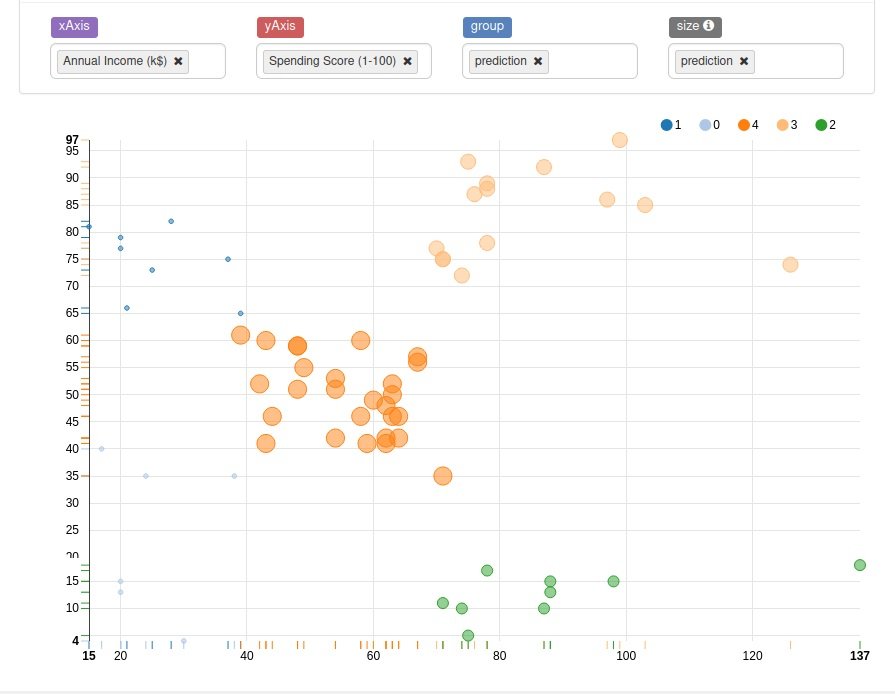
1) Cluster Set -> earning high and also spending high
2) Cluster Set ->Earning less, spending less
3) Cluster Set -> earning less but spending more
4) Cluster Set -> average in terms of earning and spending
5) Cluster Set -> earning high but spending less