Histogram for Sex and Age

%sql

select Sex,  Age from AbaloneData;

Plot Option


Age Distribution
%sql

select count(Sex), Sex from AbaloneData group by Sex;

Histogram for Lenght in mm in Abalone
%sql

select Length_in_mm from AbaloneData;

Histogram for Height in mm in Abalone
%sql

select Height_in_mm from AbaloneData;

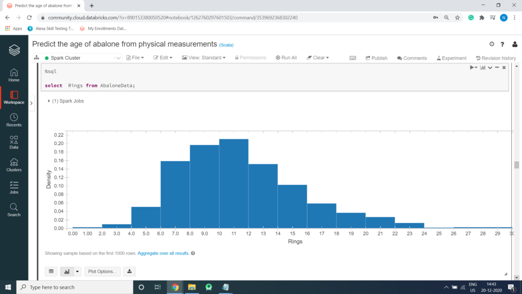
Histogram for rings in Abalone
%sql

select  Rings from AbaloneData;
Creating a Regression Model
In this tutorial , you will implement a regression model that uses features of abalone to predict the age of abalone from physical measurements
Import Spark SQL and Spark ML Libraries
First, import the libraries you will need:
%scala

import org.apache.spark.sql.functions._
import org.apache.spark.sql.Row
import org.apache.spark.sql.types._

import org.apache.spark.ml.regression.LinearRegression
import org.apache.spark.ml.feature.VectorAssembler
Prepare the Training Data
To train the Regression model, you need a training data set that includes a vector of numeric features, and a label column. In this project, you will use the VectorAssembler class to transform the feature columns into a vector, and then rename the Age column to the label.
VectorAssembler()
VectorAssembler(): is a transformer that combines a given list of columns into a single vector column. It is useful for combining raw features and features generated by different feature transformers into a single feature vector, in order to train ML models like logistic regression and decision trees.
VectorAssembler accepts the following input column types: all numeric types, boolean type, and vector type.
In each row, the values of the input columns will be concatenated into a vector in the specified order.
Collecting all String Columns into an Array
%scala

var StringfeatureCol = Array("Sex")
StringIndexer encodes a string column of labels to a column of label indices.
Example of StringIndexer
import org.apache.spark.ml.feature.StringIndexer

val df = spark.createDataFrame(
  Seq((0, "a"), (1, "b"), (2, "c"), (3, "a"), (4, "a"), (5, "c"))
).toDF("id", "category")

df.show()

val indexer = new StringIndexer()
  .setInputCol("category")
  .setOutputCol("categoryIndex")

val indexed = indexer.fit(df).transform(df)

indexed.show()

Output

+---+--------+
| id|category|
+---+--------+
|  0|       a|
|  1|       b|
|  2|       c|
|  3|       a|
|  4|       a|
|  5|       c|
+---+--------+

+---+--------+-------------+
| id|category|categoryIndex|
+---+--------+-------------+
|  0|       a|          0.0|
|  1|       b|          2.0|
|  2|       c|          1.0|
|  3|       a|          0.0|
|  4|       a|          0.0|
|  5|       c|          1.0|
+---+--------+-------------+
Define the Pipeline
A predictive model often requires multiple stages of feature preparation.
A pipeline consists of a series of transformer and estimator stages that typically prepare a DataFrame for modeling and then train a predictive model.
In this case, you will create a pipeline with stages:
- A StringIndexer estimator that converts string values to indexes for categorical features
- A VectorAssembler that combines categorical features into a single vector
%scala

import org.apache.spark.ml.attribute.Attribute
import org.apache.spark.ml.feature.{IndexToString, StringIndexer}
import org.apache.spark.ml.{Pipeline, PipelineModel}

val indexers = StringfeatureCol.map { colName =>
  new StringIndexer().setInputCol(colName).setHandleInvalid("skip").setOutputCol(colName + "_indexed")
}

val pipeline = new Pipeline()
                    .setStages(indexers)

val AbaloneFinalDF = pipeline.fit(AbaloneageDF).transform(AbaloneageDF)
Print Schema Code
%scala

AbaloneFinalDF.printSchema();

Output

root
 |-- Sex: string (nullable = true)
 |-- Length_in_mm: double (nullable = true)
 |-- Diameter_in_mm: double (nullable = true)
 |-- Height_in_mm: double (nullable = true)
 |-- Whole_in_gm: double (nullable = true)
 |-- Shucked_weight_in_gm: double (nullable = true)
 |-- Viscera_weight_in_gm: double (nullable = true)
 |-- Shell_weight_in_gm: double (nullable = true)
 |-- Rings: double (nullable = true)
 |-- Age: double (nullable = true)
 |-- Sex_indexed: double (nullable = false)
Split the Data
It is common practice when building machine learning models to split the source data, using some of it to train the model and reserving some to test the trained model. In this project, you will use 70% of the data for training, and reserve 30% for testing.
%scala

val splits = AbaloneFinalDF.randomSplit(Array(0.7, 0.3))
val train = splits(0)
val test = splits(1)
val train_rows = train.count()
val test_rows = test.count()
println("Training Rows: " + train_rows + " Testing Rows: " + test_rows)
Preparing the Training Data
%scala

import org.apache.spark.ml.feature.VectorAssembler

val assembler = new VectorAssembler().setInputCols(Array("Sex_indexed",	"Length_in_mm",	"Diameter_in_mm",	"Height_in_mm",	"Whole_in_gm",	"Shucked_weight_in_gm",	"Viscera_weight_in_gm",	"Shell_weight_in_gm", "Rings")).setOutputCol("features")

val training = assembler.transform(train).select($"features", $"Age".alias("label"))

training.show()

Output:

+--------------------+-----+
|            features|label|
+--------------------+-----+
|[2.0,0.29,0.21,0....|  7.5|
|[2.0,0.33,0.26,0....| 10.5|
|[2.0,0.335,0.22,0...|  7.5|
|[2.0,0.34,0.255,0...|  7.5|
|[2.0,0.345,0.25,0...|  7.5|
|[2.0,0.345,0.255,...| 10.5|
|[2.0,0.345,0.26,0...| 11.5|
|[2.0,0.35,0.275,0...| 11.5|
|[2.0,0.36,0.265,0...|  9.5|
|[2.0,0.36,0.265,0...| 11.5|
|[2.0,0.36,0.27,0....|  6.5|
|[2.0,0.37,0.28,0....| 11.5|
|[2.0,0.37,0.285,0...| 10.5|
|[2.0,0.37,0.29,0....| 10.5|
|[2.0,0.37,0.295,0...|  8.5|
|[2.0,0.375,0.29,0...| 11.5|
|[2.0,0.38,0.29,0....| 11.5|
|[2.0,0.38,0.3,0.0...| 10.5|
|[2.0,0.38,0.305,0...| 13.5|
|[2.0,0.38,0.325,0...| 11.5|
+--------------------+-----+
only showing top 20 rows
Train a Regression Model
Next, you need to train a regression model using the training data. To do this, create an instance of the regression algorithm you want to use and use its fit method to train a model based on the training DataFrame. In this exercise, you will use a Linear Regression algorithm – though you can use the same technique for any of the regression algorithms supported in the spark.ml API.
%scala

val lr = new LinearRegression().setLabelCol("label").setFeaturesCol("features").setMaxIter(10).setRegParam(0.3)
val model = lr.fit(training)
println("Model Trained!")
Prepare the Testing Data
Now that you have a trained model, you can test it using the testing data you reserved previously. First, you need to prepare the testing data in the same way as you did the training data by transforming the feature columns into a vector. This time you’ll rename the Age column to trueLabel.
%scala

val testing = assembler.transform(test).select($"features", $"Age".alias("trueLabel"))
testing.show()

Output:

+--------------------+---------+
|            features|trueLabel|
+--------------------+---------+
|[2.0,0.275,0.195,...|      6.5|
|[2.0,0.29,0.225,0...|      6.5|
|[2.0,0.305,0.225,...|      8.5|
|[2.0,0.305,0.23,0...|      8.5|
|[2.0,0.325,0.26,0...|      8.5|
|[2.0,0.35,0.265,0...|      8.5|
|[2.0,0.37,0.275,0...|      9.5|
|[2.0,0.37,0.275,0...|      6.5|
|[2.0,0.37,0.275,0...|      9.5|
|[2.0,0.375,0.27,0...|      8.5|
|[2.0,0.375,0.29,0...|      8.5|
|[2.0,0.375,0.295,...|      8.5|
|[2.0,0.38,0.305,0...|      9.5|
|[2.0,0.38,0.32,0....|      8.5|
|[2.0,0.39,0.29,0....|      8.5|
|[2.0,0.39,0.3,0.1...|     14.5|
|[2.0,0.395,0.295,...|     11.5|
|[2.0,0.4,0.3,0.11...|      9.5|
|[2.0,0.4,0.335,0....|     11.5|
|[2.0,0.405,0.305,...|     10.5|
+--------------------+---------+
only showing top 20 rows
Test the Model
Now you’re ready to use the transform method of the model to generate some predictions. You can use this approach to predict Age for abalone where the label is unknown; but in this case, you are using the test data which includes a known true label value, so you can compare the predicted Age.
%scala

val prediction = model.transform(testing)
val predicted = prediction.select("features", "prediction", "trueLabel")
predicted.show()

Output:

+--------------------+------------------+---------+
|            features|        prediction|trueLabel|
+--------------------+------------------+---------+
|[2.0,0.275,0.195,...| 6.686844398647028|      6.5|
|[2.0,0.29,0.225,0...| 6.738483582573759|      6.5|
|[2.0,0.305,0.225,...| 8.462873368901924|      8.5|
|[2.0,0.305,0.23,0...| 8.480795410939958|      8.5|
|[2.0,0.325,0.26,0...|  8.54065438004984|      8.5|
|[2.0,0.35,0.265,0...| 8.558666235106177|      8.5|
|[2.0,0.37,0.275,0...|  9.42241674545566|      9.5|
|[2.0,0.37,0.275,0...| 6.834284086691045|      6.5|
|[2.0,0.37,0.275,0...| 9.475088580099072|      9.5|
|[2.0,0.375,0.27,0...| 8.673248950157411|      8.5|
|[2.0,0.375,0.29,0...|  8.55209321979989|      8.5|
|[2.0,0.375,0.295,...|  8.66068301020466|      8.5|
|[2.0,0.38,0.305,0...| 9.486533208144895|      9.5|
|[2.0,0.38,0.32,0....| 8.639741397551461|      8.5|
|[2.0,0.39,0.29,0....| 8.665561785230015|      8.5|
|[2.0,0.39,0.3,0.1...|13.816461315784878|     14.5|
|[2.0,0.395,0.295,...|11.229426053517976|     11.5|
|[2.0,0.4,0.3,0.11...| 9.522982483265983|      9.5|
|[2.0,0.4,0.335,0....|11.257496662224998|     11.5|
|[2.0,0.405,0.305,...|10.358952168810188|     10.5|
+--------------------+------------------+---------+
only showing top 20 rows
Examine the Predicted and Actual Values
You can plot the predicted values against the actual values to see how accurately the model has predicted. In a perfect model, the resulting scatter plot should form a perfect diagonal line with each predicted value being identical to the actual value – in practice, some variance is to be expected.
Run the cells below to create a temporary table from the predicted DataFrame and then retrieve the predicted and actual label values using SQL. You can then display the results as a scatter plot, specifying – as the function to show the unaggregated values.
Creating Temporary View
%scala

predicted.createOrReplaceTempView("regressionPredictions")
Retrieve the Root Mean Square Error (RMSE)
There are a number of metrics used to measure the variance between predicted and actual values. Of these, the root mean square error (RMSE) is a commonly used value that is measured in the same units as the predicted and actual values –
You can use the RegressionEvaluator class to retrieve the RMSE.
%scala

import org.apache.spark.ml.evaluation.RegressionEvaluator

val evaluator = new RegressionEvaluator().setLabelCol("trueLabel").setPredictionCol("prediction").setMetricName("rmse")
val rmse = evaluator.evaluate(prediction)
println("Root Mean Square Error (RMSE): " + (rmse))

Output:

Root Mean Square Error (RMSE): 0.3000117311505641
import org.apache.spark.ml.evaluation.RegressionEvaluator
evaluator: org.apache.spark.ml.evaluation.RegressionEvaluator = RegressionEvaluator: uid=regEval_b3a7034bb1db, metricName=rmse, throughOrigin=false
rmse: Double = 0.3000117311505641